
Bayes by Backprop
Status of the notebook :
-
A working implementation of a Bayesian NN from Scratch inkl. Training by Bayes by Backprop [Blu15]
Motivation for uncertainty in the weights
According to [Blu15]
- Regularization via compression cost on the weights
- Richer representation and predictions from cheap model averaging
- Exploration in simple reinforcement learning
from [XX]
- Pruning of neural networks for reduced storage and computational cost, e.g. for mobile devices.
Bayesian Neural Networks
- instead of point estimates (MAP) we describe the weights by a probability distributions$ p(\theta) $ (see Figure 1 of [Blu15]).
- e.g. mean field approximation -$ p({\bf w}) = \prod_i p(w_i) $
- with Gaussians$ p(w_i) = \mathcal N(\mu_i, \sigma_i^2) $
Baysian Inference
- Posterior:$ p({\bf w}\mid \mathcal D) $
- Prediction:$ p({\bf \hat y} \mid {\bf \hat x}) = \mathbb E_{p({\bf w}\mid \mathcal D)}\left[p({\bf \hat y} \mid {\bf \hat x}, {\bf w})\right] $
- equivalent of using an ensemble of an uncountable infinite number of neural networks
- intractable for larger NNs
Variational Approximation
$ q({\bf w}\mid \theta) $
Minimization of the ELBO:
`DOUBLE \begin{align} \theta^* &= \text{arg} \min\theta \mathcal D{KL} \left[ q({\bf w}\mid \theta) \mid \mid p({\bf w}\mid \mathcal D)\right] \ &= \text{arg} \min\theta \mathcal D{KL} \left[ q({\bf w}\mid \theta) \mid \mid p({\bf w}) p(\mathcal D \mid \mathcal {\bf w})\right] \ &= \text{arg} \min\theta \left( \mathcal D{KL} \left[ q({\bf w}\mid \theta) \mid \mid p({\bf w}) \right]
- \mathbb E_{q({\bf w}\mid \theta)}\left[\log p(\mathcal D \mid {\bf w})\right]\right)\ \end{align} DOUBLE`
- prior dependent part / complexity cost:$ \mathcal D_{KL} \left[ q({\bf w}\mid \theta) \mid \mid p({\bf w}) \right] $
- data dependent part / likelihood cost: $ -\mathbb E_{q({\bf w}\mid \theta)}\left[\log p(\mathcal D \mid {\bf w})\right] $
import numpy as np

from matplotlib import pyplot as plt
%matplotlib inline


# we use the lightweight deep learning library dp
# you have to put dp.py in the same folder as this noebook
# you can download it from
# https://gitlab.com/deep.TEACHING/educational-materials/-/blob/master/notebooks/differentiable-programming/dp.py
# if you have downloaded the complete deep teaching git repo you find it in the folder ../differentiable-programming/

import dp # differentiable programming module
from dp import Node
# get the csv data from
# https://pjreddie.com/projects/mnist-in-csv/
#data_path = "/Users/chris/data/mnist_csv/"
data_path = "/home/chris/Downloads/"
try:
train_data_mnist
except NameError:
train_data_mnist = np.loadtxt(data_path + "mnist_train.csv", delimiter=",")
test_data_mnist = np.loadtxt(data_path + "mnist_test.csv", delimiter=",")
# TODO use standard MNIST data for faster loadingoriginal_dim = 784 # Number of pixels in MNIST images.
output_dim = nb_classes = 10 # dimensionality of the latent code z.
intermediate_dim = 128 # Size of the hidden layer.
epochs = 30
image_dim = int(np.sqrt(original_dim))
image_dimdef get_xy_mnist(data_mnist=train_data_mnist):
x = data_mnist[:,1:]
x = x / 255.
y = data_mnist[:,0]
return x, yx_train, y_train_ = get_xy_mnist()
x_test, y_test_ = get_xy_mnist(test_data_mnist)# one hot encoding for y
def one_hot_encoding(y, nb_classes=nb_classes):
m = y.shape[0]
y_ = np.zeros((m, nb_classes), dtype=int)
y_[np.arange(m), y.astype(int)] = 1
return y_
y_train = one_hot_encoding(y_train_)
y_test = one_hot_encoding(y_test_)# Standard NN
class FeedForwardNN(dp.Model):
def __init__(self, original_dim=original_dim,
intermediate_dim=intermediate_dim,
output_dim=output_dim):
super(FeedForwardNN, self).__init__()
# param
self.fc1 = self.ReLu_Layer(original_dim, intermediate_dim, "fc1")
self.fc2 = self.Linear_Layer(intermediate_dim, output_dim, "fc2")
def forward(self, x):
assert isinstance(x, Node)
h1 = self.fc1(x)
return self.fc2(h1).softmax()
def loss(self, x, y=None):
n = x.shape[0]
y_pred = self.forward(x)
loss = - y * y_pred.log()
return loss.sum()/n
batch_size=64
def random_batch(x_train=x_train, y_train=y_train, batch_size=batch_size):
    n = x_train.shape[0]
    indices = np.random.randint(0,n, size=batch_size)
    return x_train[indices], y_train[indices]
model = FeedForwardNN()x_, y_ = random_batch()
y_pred = model.forward(x=Node(x_))loss = model.loss(x=Node(x_), y=Node(y_))optimizer = dp.optimizer.RMS_Prop(model, x_train, y_train, {"alpha":0.001, "beta2":0.9}, batch_size=batch_size)
optimizer.train(steps=3000, print_each=100)iteration loss
1 2.44259090021864
100 0.3563105105925153
200 0.13585114737789328
300 0.3465467162522951
400 0.12276877525842722
500 0.24951843636899185
600 0.09596878225649089
700 0.23344820516729475
800 0.27883557784488594
900 0.1192808788147787
1000 0.10031648282381328
1100 0.09347440575806035
1200 0.11510715133199337
1300 0.06816317026451826
1400 0.142378640435843
1500 0.11166325522516689
1600 0.023504936999704743
1700 0.14019522352918665
1800 0.05362989091061093
1900 0.1336230729464381
2000 0.031242733851440187
2100 0.03128991045292066
2200 0.0401203391344262
2300 0.05551679313985189
2400 0.12693988665392572
2500 0.11841020484944927
2600 0.04701073373726761
2700 0.052503179447690604
2800 0.06533828229224387
2900 0.09233361711525746
3000 0.006093851614539158
# accuracy on train set
y_pred = model.forward(Node(x_train)).value.argmax(axis=1)
print ((y_pred==y_train_).sum()/y_train.shape[0])
0.9783
# accuracy on test set
y_pred = model.forward(Node(x_test)).value.argmax(axis=1)
print ((y_pred==y_test_).sum()/y_test.shape[0])
0.9702
Bayesian Neural Network
init_rho = -4.

# TODO: global variable
sample_store = dict()

softplus = lambda x: (1. + x.exp()).log()
NeuralNode = dp.NeuralNode


def _Linear_Bayes_Layer(fan_in, fan_out, name=None, param=dict(), initializer=None):

    assert isinstance(name, str)
    assert initializer is None # not implemented

    mu_weight_name, mu_weight_value = NeuralNode.get_name_and_set_param(param, name, "mu_weight")
    rho_weight_name, rho_weight_value = NeuralNode.get_name_and_set_param(param, name, "rho_weight")
    mu_bias_name, mu_bias_value = NeuralNode.get_name_and_set_param(param, name, "mu_bias")
    rho_bias_name, rho_bias_value = NeuralNode.get_name_and_set_param(param, name, "rho_bias")

    if mu_weight_value is None:
        mu_weight_value = NeuralNode._initialize_W(fan_in, fan_out)
        mu_bias_value = NeuralNode._initialize_b(fan_in, fan_out)
        param[mu_weight_name] = mu_weight_value
        param[mu_bias_name] = mu_bias_value

        rho_weight_value = np.ones_like(mu_weight_value) * init_rho
        rho_bias_value = np.ones_like(mu_bias_value) * init_rho
        param[rho_weight_name] = rho_weight_value
        param[rho_bias_name] = rho_bias_value

    nodes = dict()  # type: Dict[str, Node]
    def set_node(nodes, value, name):
        node = Node(value, name)
        nodes[name] = node
        return node
    W_mu = set_node(nodes, mu_weight_value, mu_weight_name)
    b_mu = set_node(nodes, mu_bias_value, mu_bias_name)
    W_rho = set_node(nodes, rho_weight_value, rho_weight_name)
    b_rho = set_node(nodes, rho_bias_value, rho_bias_name)

    def _layer(X):
        epsilon_w = np.random.normal(size=(fan_in, fan_out))
        epsilon_b = np.random.normal(size=(1, fan_out))
        W_ = W_mu + Node(epsilon_w) * softplus(W_rho)
        b_ = b_mu + Node(epsilon_b) * softplus(b_rho)

        # we need the samples for our loss
        weight_sample_name = NeuralNode._get_fullname(name, "weight_sample")
        bias_sample_name = NeuralNode._get_fullname(name, "bias_sample")
        sample_store[weight_sample_name] = W_
        sample_store[bias_sample_name] = b_
        return X.dot(W_) + b_

    return _layer, param, nodes


def Linear_Bayes_Layer(self, fan_in, fan_out, name=None):
    return self._set_layer(fan_in, fan_out, name, _Linear_Bayes_Layer)

setattr(dp.Model, "Linear_Bayes_Layer", Linear_Bayes_Layer)
class BayesFeedForwardNN(dp.Model):
def __init__(self, original_dim=original_dim,
intermediate_dim=intermediate_dim,
output_dim=output_dim):
super(BayesFeedForwardNN, self).__init__()
# param
self.fc1 = self.Linear_Bayes_Layer(original_dim, intermediate_dim, "fc1")
self.fc2 = self.Linear_Bayes_Layer(intermediate_dim, output_dim, "fc2")
def forward(self, x):
assert isinstance(x, Node)
h1 = self.fc1(x).relu()
return self.fc2(h1).softmax()
def loss(self, x, y=None):
raise NotImplementedError()
`DOUBLE \begin{align} \theta^* &= \text{arg} \min\theta \left( \mathcal D{KL} \left[ q({\bf w}\mid \theta) \mid \mid p({\bf w}) \right]
- \mathbb E{q({\bf w}\mid \theta)}\left[\log p(\mathcal D \mid {\bf w})\right]\right)\ &= \text{arg} \min\theta \left( \mathbb E{q({\bf w}\mid \theta)}\left[ \log q({\bf w}\mid \theta)\right]- \mathbb E{q({\bf w}\mid \theta)}\left[\log p({\bf w})\right]
- \mathbb E_{q({\bf w}\mid \theta)}\left[\log p(\mathcal D \mid {\bf w})\right]\right)\ \end{align} DOUBLE`
So equivalently we want to minimize the following loss:
`DOUBLE loss = \mathbb E{q({\bf w}\mid \theta)}\left[\log q({\bf w}\mid \theta)\right]- \mathbb E{q({\bf w}\mid \theta)}\left[ \log p({\bf w})\right]
- \mathbb E_{q({\bf w}\mid \theta)}\left[\log p(\mathcal D \mid {\bf w})\right] DOUBLE`
Entropy
$ \mathbb E_{q({\bf w}\mid \theta)}\left[ \log q({\bf w}\mid \theta)\right] $
Note: That's the negative entropy of$ q({\bf w}\mid \theta) $. So this terms tries to maximize the entropy of$ q $.
We can compute the expectations by Monte-Carlo estimates.
So we sample for each data point$ l $ of a mini-batch a sample from the variational distribution:
$ {\bf w}^{(l)} \sim q({\bf w}\mid \theta) $
-$ l \in [1, 2, \dots, m] $ -$ m $ number of data points in the mini-batch -$ n $ total number of data points
Then we have for the approximated loss in the mini-batch: $ loss_{mb} \approx \frac{m}{n}\sum_{l=1}^m \log q({\bf w}^{(l)}\mid \theta)- \frac{m}{n}\sum_{l=1}^m \log p({\bf w}^{(l)}) - \sum_{l=1}^m\log p({\bf y}^{(l)} \mid {\bf w}^{(l)}, {\bf x}^{(l)}) $
negative Log-Likelihood
`DOUBLE
- \sum_{l=1}^m\log p({\bf y}^{(l)} \mid {\bf w}^{(l)}, {\bf x}^{(l)}) DOUBLE`
Log-Posterior
$ \frac{m}{n} \sum_{l=1}^m \log q({\bf w}^{(l)}\mid \theta) $
PI_2 = 2.0 * np.pi
LOG_PI_2 = float(np.log(PI_2))

def log_normal(sample, mu, sigma):
    return - 0.5 * LOG_PI_2 - sigma.log() - (sample-mu).square() / (2.*sigma.square())
Log-Prior
`DOUBLE
- \frac{m}{n} \sum_{l=1}^n \log p({\bf w}^{(l)}) DOUBLE`
Mean-Field approximation: $ \log p({\bf w}^{(l)}) = \sum_i\log p(w_i^{(l)}) $
with Gaussian-Priors:
$ p(weight_i) = \mathcal N(weight_i \mid 0,\sigma_{weight}^2) $
$ p(bias_j) = \mathcal N(bias_j \mid 0,\sigma_{bias}^2) $
# scale mixture prior
def normal(w, var, mu=0):
    s = 1.0 / np.sqrt(PI_2 * var)
    g = (- (w - mu).square() / (2 * float(var))).exp()
    return s * g

var_g1 = np.exp(-1.)**2
var_g2 = np.exp(-7.)**2
p = 0.25
def log_scale_mixture_prior(w, var_g1=var_g1, var_g2=var_g2):
    first = p * normal(w, var_g1)
    second = (1 - p) * normal(w, var_g2)
    return (first + second).log()
# Hyperparameter
sigma = Node(0.5)
M = x_train.shape[0]/batch_size# num. of batches
def loss(self, x, y):# TODO: nb_batched should be given as argument
m = x.shape[0]
y_pred = self.forward(x)
# y must be one hot encoded
assert (y.shape == y_pred.shape)
# data likelihood - here cross-entropy
neg_log_likelihood = - (y * y_pred.log()).sum()
# prior
log_prior = 0
for sample_name, sample_value in sample_store.items():
if sample_name.endswith("_sample"):
#log_prior += log_normal(sample_value, 0., sigma).sum()
log_prior += log_scale_mixture_prior(sample_value).sum()
#variational posterior
log_posterior = 0.
for nnode_name, nnode_value in self.neural_nodes.items():
nn = nnode_name.split("_")
sample_weight = sample_store[nn[0]+"_weight_sample"]
sample_bias = sample_store[nn[0]+"_bias_sample"]
for node_name, node_value in nnode_value.nodes.items():
if node_name.endswith("mu_weight"):
mu_weight = node_value
if node_name.endswith("mu_bias"):
mu_bias = node_value
if node_name.endswith("rho_weight"):
rho_weight = node_value
if node_name.endswith("rho_bias"):
rho_bias = node_value
log_posterior += log_normal(sample_weight, mu_weight, softplus(rho_weight)).sum()
log_posterior += log_normal(sample_bias, mu_bias, softplus(rho_bias)).sum()
# TODO different weighting of complexity vd data cost during training
# see paper 3.4.
loss_ = neg_log_likelihood + 1/M*(log_posterior - log_prior)
return loss_
BayesFeedForwardNN.loss = lossbayes_model = BayesFeedForwardNN()optimizer = dp.optimizer.RMS_Prop(bayes_model, x_train, y_train,
{"alpha":0.001, "beta2":0.9},
batch_size=batch_size)
optimizer.train(steps=10000, print_each=100)iteration loss
1 555.8524743339495
100 432.19328154564505
200 425.5282834927088
300 399.7855085185947
400 388.1594144420811
500 381.9412499799676
600 385.74467175502974
700 386.5106035931867
800 375.8686212840836
900 382.0504437684173
1000 376.279215690231
1100 365.2414078904296
1200 368.46763266460977
1300 373.29237033984776
1400 366.15632683246065
1500 359.5466638302649
1600 359.9014343186206
1700 355.3065088551375
1800 350.5585995305178
1900 350.9459805287687
2000 343.48580990549965
2100 346.8447042158543
2200 341.12262461199634
2300 346.77652392774763
2400 336.1143906573853
2500 341.75459864389205
2600 344.6684848241343
2700 338.0187913673604
2800 330.91542750706253
2900 330.79186976649885
3000 336.3696240521043
3100 323.4057671181288
3200 337.49009462579403
3300 324.85056015522173
3400 324.4397445491907
3500 319.50658121097536
3600 325.44405122044145
3700 312.13655154264427
3800 311.7469325216087
3900 309.16729680392643
4000 308.5556604191104
4100 306.05650332097207
4200 309.97855270890955
4300 303.230174740776
4400 313.0212910641261
4500 296.3730682049053
4600 294.1913345613057
4700 293.3870182234443
4800 291.00676672249574
4900 292.9634531771089
5000 290.7470633403903
5100 289.5400624775794
5200 294.2945232297104
5300 282.7186033579018
5400 277.9272590949305
5500 280.47359964227235
5600 275.6599734576633
5700 272.6786374603832
5800 274.1234111397373
5900 270.58702263454455
6000 270.3045527272958
6100 270.80812968372027
6200 263.52604545639235
6300 265.99153401652933
6400 257.5574445410981
6500 256.4176346100624
6600 252.3497648491807
6700 255.1209298509782
6800 250.6626107619079
6900 253.66572698749567
7000 246.2654606405229
7100 246.43371278441495
7200 244.71832271550056
7300 243.38126570585783
7400 237.67298392804992
7500 236.48316562078
7600 234.29633576071845
7700 239.84568010804318
7800 231.40301653931675
7900 230.3234800528206
8000 243.0108008006537
8100 227.80015415791308
8200 232.81771053313645
8300 228.7706050735224
8400 233.4289043358385
8500 227.81839664238365
8600 223.07728741898333
8700 221.9306857638958
8800 220.76133921376731
8900 227.0592752719502
9000 218.94043683919875
9100 224.61937781453324
9200 216.39602376307548
9300 215.2404214852406
9400 216.42226419684224
9500 213.5575270615868
9600 210.940764736489
9700 215.79251639547186
9800 212.38041028005614
9900 215.0095979811585
10000 209.60373750918436
y_pred = bayes_model.forward(Node(x_test)).value
y_pred = y_pred.argmax(axis=1)
(y_pred == y_test_).sum()/y_test_.shape[0]
The expectation can be approximated by $ p({\bf \hat y} \mid {\bf \hat x}) \approx \mathbb E_{q({\bf w}\mid \mathcal D)}\left[p({\bf \hat y} \mid {\bf \hat x}, {\bf w})\right] $
MC-Estimate:
$ p({\bf \hat y} \mid {\bf \hat x}) \approx \mathbb \sum_{{\bf w}'}p({\bf \hat y} \mid {\bf \hat x}, {\bf w'}) $
y_preds = []
for i in range(10):
    y_preds.append(bayes_model.forward(Node(x_test)).value)
y_preds = np.array(y_preds)
y_pred = y_preds.mean(axis=0)
y_pred = y_pred.argmax(axis=1)
(y_pred == y_test_).sum()/y_test_.shape[0]# uncertainty of the max_pred
y_uncertainty = y_preds.std(axis=0)# the most uncertained
i=y_uncertainty[range(len(y_uncertainty)),y_pred].argmax()
plt.figure()
plt.imshow(x_test[i].reshape(28, 28), cmap='gray')
plt.show()
print(y_preds.mean(axis=0)[i].max())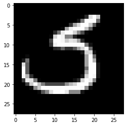
0.5789877528566475
i = y_preds.mean(axis=0)[range(len(y_pred)), y_pred].argmin()
print(y_pred[i])
5
# the lowest class prediction max
plt.figure()
plt.imshow(x_test[i].reshape(28, 28), cmap='gray')
plt.show()
print(y_preds.mean(axis=0)[i].max())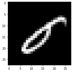
0.23103863529292376
Literature
- [Blu15] Charles Blundell, Julien Cornebise, Koray Kavukcuoglu, Daan Wierstra: Weight Uncertainty in Neural Networks, https://arxiv.org/abs/1505.05424