
Status: Draft
Medical Image Classification Scenario
This project contains Python Jupyter notebooks to teach machine learning content in the context of medical data, e.g., automated tumor detection. The material focuses primarily on teaching basic knowledge of convolutional neural networks but also contains portions of fundamental machine learning knowledge.
1) Scenario Description
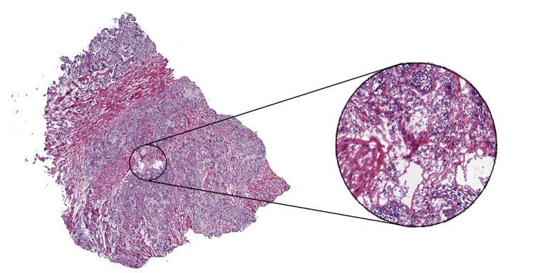
To determine the exact state of breast cancer and therefore subsequent therapy decisions, it is essential to analyze a patient’s tissue samples under a microscope. Examining such tissue slides is a complex task that requires years of training and expertise in a specific area by a pathologist. But scientific studies show that even in a group of highly experienced experts there can be substantial variability in the diagnoses for the same patient, which indicates the possibility of misdiagnosis [ELM15][ROB95]. This result is not surprising given the enormous amount of details in a tissue slide at 40x magnification. To get a sense of the amount of data, imagine that an average digitized tissue slide has a size of 200.000x100.000 pixel and you have to inspect every one of them to get an accurate diagnose. Needless to say, if you have to examine multiple slides per patient and have several patients, this is a lot of data to cover in a usually limited amount of diagnosis time. Following image depicts a scanned tissue slide (whole slide image, short WSI) at different magnification level.
Under such circumstances, an automated detection algorithm can naturally complement the pathologists’ work process to enhance the possibility of an accurate diagnosis. Such algorithms have been successfully developed in the scientific field in recent years, in particular, models based on convolutional neural networks [WAN16][LIU17]. But getting enough data to train machine learning algorithms is still a challenge in the medical context. However, the Radboud University Medical Center (Nijmegen, the Netherlands) and the University Medical Center Utrecht (Utrecht, the Netherlands) provide an extensive dataset containing sentinel lymph nodes of breast cancer patients in the context of their CAMELYON challenge. These data provide a good starting point for further scientific investigations and are therefore mainly used in that scenario. You can get the data at CAMELYON17 challenge (GoogleDrive/Baidu).
In context of the medical scenario you will develop a custom classifier for the given medical dataset that will decide:
- If a lymph node tissue contains metastases.
- What kinds of metastases are present, e.g., micro- or macro-metastasis (see here)?
- Which pN-stage the patient is in, based on the TNM staging system?
1.1) Teaching Material
Detection of metastases is a classification problem. To solve this first issue, you will implement a classification pipeline based on convolutional neural network (CNN)[LEC98]. Further, you will extend that pipeline with classical machine learning approaches, like decision trees, to address the second and third issue.
We divide the teaching material in that scenario into:
-
WSI preprocessing:
- Introduction into handling of WSI data.
- Dividing WSIs into smaller tiles.
- Creating a fast accessible data set of tiles for training a cnn.
-
Tile classification:
- Training a cnn to predict whether a tile contains metastases or not.
- Prediction / Assigning a score between 0.0 and 1.0 to each tile of the WSIs in the test set.
- Combining all prediction results of a WSI to form a heatmap.
-
WSI classification:
- Manually extract features of the heatmaps, like are of the biggest region of high confidence (score).
- Training a decision tree with extracted features.
- Predicting each slide if it contains no metastases, itcs, micro metastases or macro metastases.
-
pN-stage classification:
- Assigning the pN-stage to each patient in the test set based on the predicted labels (itc, micro, …) of his WSIs.
- Calculating the weighted kappa score for the pN-stage predictions test set.
The deep.TEACHING project provides educational material for students to gain basic knowledge about the problem domain, the programming, math and statistics requirements, as well as the mentioned algorithms and their evaluation. Students will also learn how to construct complex machine learning systems, which can incorporate several algorithms at once.
2) Medical Background
Read this section to get more information on the medical backround. Profound understanding of the domain and the problem we are working on is fundamental to efficiently apply machine learning algorithms to solve the problem.
To determine the exact state of breast cancer and therefore subsequent therapy decisions, it is essential to analyze a patient’s tissue samples under a microscope. The tissue was extracted from lymph nodes of the breast region. Examining lymph nodes is crucial in case of breast cancer, as they are the first place breast cancer is likely to spread to. The tissue is fixed between two small glass plates, which is called slide. After digitizing of those slides, we call them whole-slide-images (WSIs).
2.1) pN-Stage
How badly and how many lymph nodes are infested determines the pN-stage of the patient. In other words, the pN-stage quantifies the infestation of the lymph nodes.
The stage pN2 for example means, that metastases were found in at least 4 nodes, of which at least one is a macro-metastasis. The CAMELYON17 challenge distinguishes five different pN-stages. For a detailed description see the evaluation section of the CAMELYON17 website.
2.2) Slide Labels
A slide can contain no tumorous tissue at all (class label negative), contain only a very small tumorous area (isolated tumor cells, short itc), a small to medium area (micro metastases) or a bigger area of tumorous tissue (macro metastses). See also evaluation section.
2.3) Data Set
The data set we are going to use is the CAMELYON data set. It is divided into two sub data sets. See also the data section of the CAMELYON website.
CAMELYON16
The training set contains 270 WSIs. They are not labeled with negative, itc, micro or macro. Their labels are only positive (contains metastases) or negative. Additionally xml files are provided for positive slides, which contain coordinates for polygons to describe the metastatic regions.
The test set contains 130 WSIs, also with xml files. At the beginning of the CAMELYON17 challenge, the WSIs of the test set additionally received the labels negative, itc, micro or macro, though no examples for the itc class are included.
CAMELYON17
The training and the test set contain each 100 patients. One patient consists of 5 WSIs, which are labeled with negative, itc, micro or macro, but only the labels of the training set are publicly available.
3) Requirements
ATTENTION: The first half of the notebooks, which are about WSI preprocessing and Tile Classification require at least 3.5 tera bytes space for the data set, and a fairly strong GPU (at least Geforce 1070 recommended), and a lot of time to run the processes.
If you cannot provide these hardware requirements, you can directly jump to WSI classification, where you will be provided with a sample solution to go on from there. All subsequent notebooks do not require a GPU or anymore than several hundred mega bytes.
To run the first half of the notebooks, you will also need to install openslide, which is needed to read the WSIs tif format.
If you decide to directly start with WSI classification, we still suggest to read through everything on this page as well as the jupyter notebooks for WSI preprocessing and Tile Classification, as it will provide you with the big picture of the data processing pipeline.
3.A) Install using Conda (Recommended - Tested on Ubuntu 18.04)
3.A) Conda Install - Openslide and Python Packages
Using Conda on Ubuntu 18.04 (Tested):
Use the following commands to create and activate a conda environment:
conda create -n myenv
conda activate myenv
Then install the following packages via pip/conda (note to NOT use the --user flag for pip install inside a conda env!
conda install scipy=1.3.1
conda install tensorflow-gpu=1.14
conda install -c bioconda openslide=3.4.1
conda install -c conda-forge libiconv=1.15
conda install -c bioconda openslide-python==1.1.1
conda install python-graphviz=0.13.2
pip install openslide-python==1.1.1
pip install progress==1.5
pip install scikit-image==0.16.2
pip install scikit-learn==0.21.3
pip install pandas=0.25.3
3.B) Manual Install (Tested on Ubuntu 18.04)
3.B) Manual Install - Openslide
Manually on Ubuntu 18.04 (Tested):
-
Go to the openslide download page and download the tar.gz
- This tutorial uses openslide version 3.4.1, which is confirmed to work (2018-11-02).
-
Install the following system packages. It is suggested to install the newest versions with:
sudo apt-get install libjpeg-dev libtiff-dev libglib2.0-dev libcairo2-dev ibgdk-pixbuf2.0-dev libxml2-dev libsqlite3-dev valgrind zlib1g-dev libopenjp2-tools libopenjp2-7-dev python3-dev -
However, if installation fails, the following versions are confirmed to work with openslide version 3.4.1:
sudo apt-get install libjpeg-dev=8c-2ubuntu8 libtiff-dev=4.0.9-5 libglib2.0-dev=2.56.2-0ubuntu0.18.04.2 libcairo2-dev=1.15.10-2 ibgdk-pixbuf2.0-dev=2.36.11-2 libxml2-dev=2.9.4+dfsg1-6.1ubuntu1.2 libsqlite3-dev=3.22.0-1 valgrind=1:3.13.0-2ubuntu2.1 zlib1g-dev=1:1.2.11.dfsg-0ubuntu2 libopenjp2-tools=2.3.0-1 libopenjp2-tools=2.3.0-1 libopenjp2-7-dev=2.3.0-1 python3-dev -
Unpack the openslide
tar.gzfile and inside the unpacked folder execute the following (excerpt from the README.txt):./configure make make install -
Finally add the following to the end of your ~/.bashrc
########## OpenSlide START ############
LD_LIBRARY_PATH=${LD_LIBRARY_PATH}:/usr/local/lib
export LD_LIBRARY_PATH
########## OpenSlide END ##############
3.B) Manual Install - Python Packages
Install the corresponding python packages (see 3.A).
4) Teaching Content and Exercises
Read this section for an overview of the data processing pipeline and the workflow covered in the notebooks. At the end of a subsection, exercise-notebooks are linked:
- There are exercise-notebooks, which work with the original medical data (marked with specific). These exercise-notebooks are meant to be completed in chronological order, since one might require the results of the preceding exercise.
- There also exist more generic notebooks which are about the same machine-learning technique, but work with artificial data and can be completed as stand-alone exercises. These notebooks are marked with generic.
4.1) WSI preprocessing
With an average size of 200.000 x 100.000 pixels per WSI at the highest zoom level, it is impossible to directly train a CNN to predict the labels negative, itc, micro or macro. Therefore, the problem has to be divided into sub tasks. At the end of a sub task, the jupyter notebook containing the corresponding exercise is linked. The WSIs are divided into smaller pieces (tiles) with a fixed size, e.g. 256 x 256 pixels. Each tiles is labeled with positive or negative.
The first notebook does not yet include exercises. Have a look at it to get an idea how to possibly write a wrapper for openSlide accessing the WSI-Tiff format.
- data-handling-usage-guide.ipynb - specific
The most time is consumed when we access a specific area of a WSI in a specific magnificaiton level. Therefore it is a good idea to create a custom dataset of the WSIs in the training set to efficiently access batches of tiles.
- create-custom-dataset.ipynb - specific
4.2) Tile classification
Color normalization and data augmentation is all used inside the notebook of subsection (4.2.3) where you will train a CNN. Though before we proceed with that, you should know why this is might be needed and how it works in general.
Color Normalization
There exist two reasons, why color normalization is crucial:
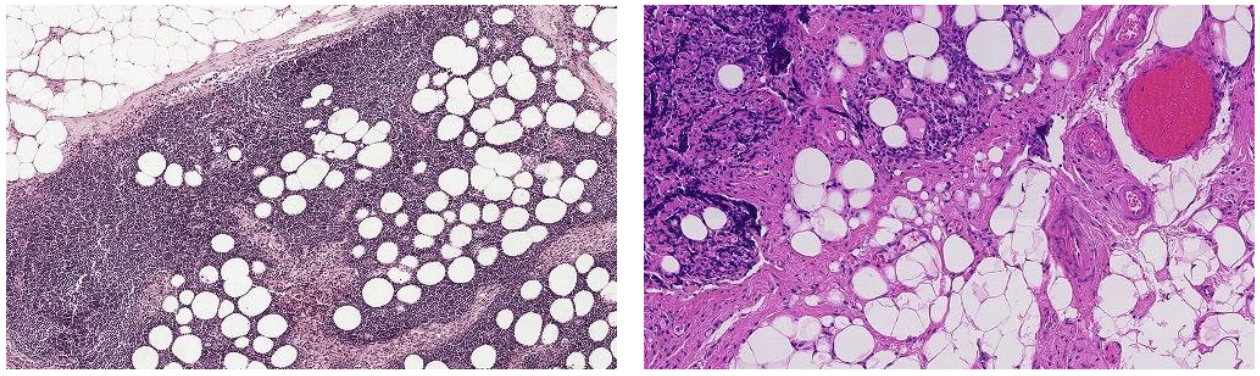
- The chemicals used to colorize a WSI (staining process) can slightly differ resulting in very different colors.
- Different slide scanners used to digitize the slides. Below you can see parts of two different slides, varying greatly in color.
Data Augmentation
There are a lot more negative tiles than positive ones. And as always in the context of machine learning, more data to train on is never bad. Common data augmentation techniques are mirroring, rotation, cropping and adding noise.
- exercise-images-data-augmentation-numpy - generic
Training a CNN
With normalized and augmented tiles, we can train a CNN to predict whether a tile contains metastases or not.
- exercise-train-cnn-tensorflow - specific
For an in-depth understanding about convolutional neural networks, we recommend working through the course Convolutional Neural Network.
Heatmap creation
The output of the CNN is a confidence score from 0.0 to 1.0, whether a tile contains metastases. The score of the individual tiles of a WSI can then be used to create a confidence map (or heatmap). Here are some examples for such heatmaps. The brighter a pixel the higher the confidence for metastates. White being very high confidence.
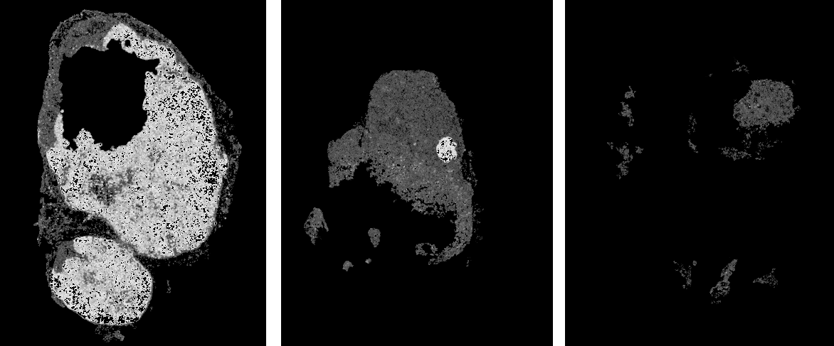
- exercise-prediction-and-heatmap-generation - specific
4.3) WSI classification
Feature Extraction
Unfortunately the training data here is very limited as we have only 500 slides from the CAMELYON17 training set and 130 labled slides from the CAMELYON16 test set (labled with negative, itc, micro, macro). So opposed to the task of the CAMELYON16 challenge where we had thousands of tiles and only two different labels (normal and tumor), we will not be able to supply another CNN model with sufficient data. Even worse, for the itc class, we only have 35 examples in total.
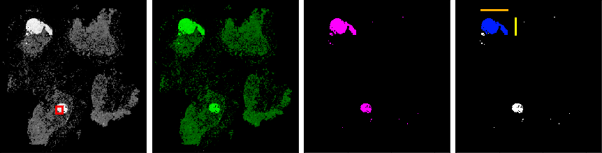
To tackle this problem, our approach is to make use of domain specific knowledge and extract geoemtrical features from the heatmaps, which can be used to train a less complex model, like a decision tree. Possible features are:
- Highest probability (value) on the heatmap (red)
- Average probability on the heatmp. Sum all values and divide by the number of values $\gt 0.0$ (green)
- Number of pixels after thresholding (pink)
- Length of the larger side of the biggest object after thresholding (orange)
- Length of the smaller side of the biggest object after thresholding (yellow)
- Number of pixels of the biggest object after thresholding (blue)
- exercise-extract-features - specific
Training a Decision Tree
With the extracted features we can train another classifier to predict whether a WSI contains no metastases (negative), only small area of metastases (itc), medium sized metastases (micro) or a bigger region (macro). A possible classifier for this task would be a decision tree, a random forest, a support vector machine, naive bayes or even a multi layer perceptron (fully connected feed forward network).
- exercise-decision-trees - generic
- exercise-entropy - generic
- exercise-classify-heatmaps - specific
4.4) pN-Stage classification
When all 5 slides of a patient are predicted with negative, itc, micro or macro, we can classify the patient’s pN-stage by just applying the simple rules found at the evaluation section of the CAMELYON17 website. After that you can calculate the score and compare your results with the official submission on the CAMELYON challenge results page. However, note that your results are based on the training set, whereas the official submissions are based on the CAMEYLON17 test set. If you apply your classifier on the test set, expect like 5-10% lower kappa score.
- exercise-evaluation-metrics - generic
- exercise-calculate-kappa-score - specific
Reference (ISO 690)
| [ELM15] | ELMORE, Joann G., et al. Diagnostic concordance among pathologists interpreting breast biopsy specimens. Jama, 2015, 313. Jg., Nr. 11, S. 1122-1132. |
| [LEC98] | LeCun, Yann, et al. "Gradient-based learning applied to document recognition." Proceedings of the IEEE 86.11 (1998): 2278-2324. |
| [LIU17] | LIU, Yun, et al. Detecting cancer metastases on gigapixel pathology images. arXiv preprint arXiv:1703.02442, 2017. |
| [ROB95] | ROBBINS, P., et al. Histological grading of breast carcinomas: a study of interobserver agreement. Human pathology, 1995, 26. Jg., Nr. 8, S. 873-879. |
| [WAN16] | WANG, Dayong, et al. Deep learning for identifying metastatic breast cancer. arXiv preprint arXiv:1606.05718, 2016. |